5.3 Program Relax

5.3.1 Purpose

relax drives and controls a non-linear optimization procedure to locate the minimum (or a stationary point) of a function f(x). In TURBOMOLE f is always the electronic energy, and the coordinates x will be referred to as general coordinates. They include

• cartesian atomic coordinates
• internal atomic coordinates
• exponents, contraction coefficients and scaling factors of basis functions
• a global scaling factor (a common scaling factor for all basis set exponents)

The optimization employs an iterative procedure based on gradients ∇f of the current and, if available, previous iterations. Various procedures can be applied: steepest descent, Pulay’s DIIS, quasi–Newton, conjugate gradients, as well as combinations of them. relax carries out:

• update of general coordinates
• update of approximate hessians if needed
• conversion of coordinates (internal ←→ cartesian)

The mode of operation is chosen by the keywords $optimize and $interconversion and the corresponding options, which will be described in the following sections.

5.3.2 Optimization of General Coordinates

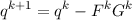
After gradients G^k have been calculated for coordinates q^k in optimization cycle k, new coordinates (or basis set exponents) q^k+1 can be obtained from the quasi–Newton update:

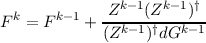
where F^k is the inverse of an approximate force constant matrix H^k. This method would immediately converge to the equilibrium geometry if F^k would be the inverse of the exact force constant matrix and the force field would be quadratic. In real applications usually none of these requirements is fulfilled. Often only a crude approximation to the force constant matrix H^k is known. Sometimes a unit matrix is employed (which means coordinate update along the negative gradient with all coordinates treated on an equal footing).

The optimization of nuclear coordinates in the space of internal coordinates is the default task performed by relax and does not need to be enabled. Any other optimization task requires explicit specifications in data group $optimize, which takes several possible options:

$optimize options

internal on/off

Structure optimization in internal coordinates.

redundant on/off

Structure optimization in redundant coordinates.

cartesian on/off

Structure optimization in cartesian coordinates.

basis on/off

Optimization of basis set exponents, contraction coefficients, scaling factors.

global on/off

Optimization of global scaling factor for all basis set exponents.

Note: All options except internal are switched off by default, unless they have been activated explicitly by specifying on.

Some of the options may be used simultaneously, e.g.

• internal, basis
• internal, global
• cartesian, basis

Other options have to be used exclusively, e.g.

• internal, cartesian
• basis, global

The update of the coordinates may be controlled by special options provided in data group $coordinateupdate which takes as options:

dqmax=real

Maximum total coordinate change (default: 0.3).

interpolate on/off

Calculate coordinate update by inter/extrapolation using coordinates and gradients of the last two optimization cycles (default: interpolate on) if possible.

statistics integer/off

Display optimization statistics for the integer previous optimization cycles. Without integer all available information will be displayed. off suppresses optimization statistics.

The following data blocks are used by program relax:

1.

Input data from gradient programs grad, rdgrad, egrad, rimp2, mpgrad, etc.:

$grad

cartesian atomic coordinates and their gradients.

$egrad

exponents and scale factors and their gradients.

$globgrad

global scale factor and its gradient.

2.

Input data from force constant program aoforce:

$grad

cartesian atomic coordinates and their gradients.

$globgrad

global scale factor and its gradient.

$hessian

the force constant matrix in the space of cartesian coordinates.

3.

Output data from program relax:

$coord

cartesian atomic coordinates.

$basis

exponents and scale factors.

$global

global scale factor.

For structure optimizations the use of (redundant) internal coordinates is recommended, see Section 4.0.6. Normally internal coordinates are not used for input or output by the electronic structure programs (dscf, mpgrad, etc.). Instead the coordinates, gradients, etc. are automatically converted to internal coordinates by relax on input and the updated positions of the nuclei are written in cartesians coordinates to the data group $coord. Details are explained in the following sections.

5.3.3 Force Constant Update Algorithms

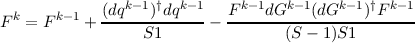
In a Newton-type geometry update procedure often only a crude approximation to the force constant matrix H^k is available. What can be done then is to update F^k = (H^k)^-1 in each iteration using information about previous coordinates and gradients. This constitutes the quasi–Newton or variable metric methods of which there are a few variants:

1.

Murtagh/Sargent (MS):

2.

Broyden/Fletcher/Goldfarb/Shanno (BFGS):

3.

Davidon/Fletcher/Powell (DFP):

4.

combined method (BFGS/DFP): If S1 < (S - 1)S1 and S1 > 0 perform DFP update, otherwise BFGS.

The meaning of the symbols above is as follows:

F^k = (H^k)^-1

approximate inverse force constant matrix in the k-th iteration.s

q^k

general coordinates in the k-th iteration.

G^k

gradients in the k-th iteration.

dq^k-1 = q^k - q^k-1

dg^k-1 = g^k - g^k-1

Z^k-1 = dq^k-1 - F^k-1dG^k-1

S1 = (dq^k-1)^†dg^k-1

S = 1 + ((dg^k-1)^†F^k-1dG^k-1)∕(S1)

An alternative is to use update algorithms for the hessian H^k itself:

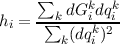
Ehrig, Ahlrichs : Diagonal update for the hessian by means of a least squares fit

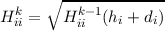with the new estimate h for the diagonal elements obtained by

and the error d obtained by the regression

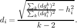Another alternative is to use DIIS-like methods: structure optimization by direct inversion in the iterative subspace. (See ref.  [37] for the description of the algorithm). The DIIS procedure can often be applied with good success, using static or updated force constant matrices.

Any of the algorithms mentioned above may be chosen. Recommended is the macro option ahlrichs, which leads to the following actions (n is the maximum number of structures to be included for the update, default is n = 4):

ncycles < n:  

geometry update by inter/extrapolation using the last 2 geometries.

ncycles ≥ n:  

diagonal update for the hessian as described above; DIIS–like update for the geometry.

||G|| < thr:  

BFGS-type update of the hessian and quasi–Newton update of (generalized) coordinates.

References for the algorithms mentioned above: [34,37–41]

5.3.4 Definition of Internal Coordinates

If structure optimizations are to be performed in the space of internal coordinates ($optimize internal, is the default setting), appropriate internal coordinate definitions have to be provided on data block $intdef. The types available and their definitions are described in Section 4.1.2. For recommendations about the choice of internal coordinates consult ref. [28]. Nevertheless the structure of $intdef will shortly be described. The syntax is (in free format):

The first items have been explained in Chapter 4.

Two additional items val=real, fdiag=real may be supplied for special purposes:

val=

serves for the input of values for internal coordinates for the interconversion internal → cartesian coordinates; it will be read in by relax if the flag for interconversion of coordinates has been activated ($interconversion on ), or by the interactive input program define within the geometry specification menu.

fdiag=

serves for the input of (diagonal) force constants for the individual internal coordinates to initialize $forceapprox.

5.3.5 Structure Optimizations Using Internal Coordinates

This is the default task of relax ($optimize internal on does not need to be specified!) You need as input the data groups :

$grad

cartesian coordinates and gradients as provided and accumulated in subsequent optimization cycles by the programs grad, or rdgrad etc.

$intdef

definitions of internal coordinates.

$redundant

definitions of redundant coordinates.

Output will be the updated coordinates on $coord and the updated force constant matrix on $forceapprox. If any non-default force constant update option has been chosen, relax increments its counting variables <numgeo>, <numpul> within command keyword $forceupdate. If the approximate force constant has been initialized ($forceinit on ) relax switches the initialization flag to $forceinit off. Refer also to the general documentation of TURBOMOLE. It is recommended to check correctness of your definition of internal coordinates:

1.

Calculate their values for your cartesian start coordinates using the relax program (see Section 5.3.11) or within a define session.

2.

Have a look at the eigenvectors of the BmB^†-matrix. Set some ‘?’ behind keyword $intdef, if there are any eigenvalues close to zero (< 10^-2 is to be considered bad for small molecules, but there is no general rule) check those internal coordinates for consistency which contribute to the corresponding eigenvector(s)!

5.3.6 Structure Optimization in Cartesian Coordinates

For this task you have to specify:

These lines switch on the non-default optimization in cartesian coordinates and switch off the optimization in internal coordinates (this has to be done explicitly!). As input data groups you need only $grad as provided by on of the gradient programs. For the first coordinate update an approximate force constant matrix is needed in data group $forceapprox. Output will be the updated coordinates on $coord, and the updated force constant matrix on $forceapprox.

The coordinates for any single atom can be fixed by placing an ’f’ in the third to eighth column of the chemical symbol/flag group. As an example, the following coordinates specify acetone with a fixed carbonyl group:

5.3.7 Optimization of Basis Sets (SCF only)

For this task you have to specify:

This example would perform only a basis set optimization without accompanying geometry optimization. It is possible, of course, to optimize both simultaneously: Just leave out the last line of the example (internal off). Input data groups are:

$egrad

Basis set exponents, contraction coefficients, scaling factors and their respective gradients as provided and accumulated in subsequent optimization cycles by one of the programs grad or mpgrad, if $drvopt basis on has been set.

$basis

Description of basis sets used, see Section 4.2.

Output will be the updated basis on $basis, and the updated force constant matrix on $forceapprox.

For an example, see Section 21.5.

5.3.8 Simultaneous Optimization of Basis Set and Structure

The optimization of geometry and basis set may be performed simultaneously and requires the specification of:

and needs as input data groups $grad and $egrad. Output will be on $coord, $basis, also on $forceapprox (updated).

5.3.9 Optimization of Structure and a Global Scaling Factor

Optimization of a global scaling factor is usually not performed in geometry optimizations. It is a special feature for special applications by even more special users. As reference see [42].

To optimize the structure and a global scaling factor specify:

You need as input data groups $grad and $globgrad, the latter contains the global scaling factors and their gradients accumulated in all optimization cycles. Output will be on $coord, $global, also on $forceapprox (updated). Note that for optimization of a global scaling factor a larger initial force constant element is recommended (about 10.0).

5.3.10 Conversion from Internal to Cartesian Coordinates

Due to translational and rotational degrees of freedom and the non-linear dependence of internal coordinates upon cartesian coordinates, there is no unique set of cartesian coordinates for a given set of internal coordinates. Therefore an iterative procedure is employed to calculate the next local solution for a given cartesian start coordinates. This task may be performed using the relax program, but it is much easier done within a define session.

5.3.11 Conversion of Cartesian Coordinates, Gradients and Force Constants to Internals

To perform this tasks, you have to activate the interconversion mode by

Note that any combination of the three options showed is allowed! The default value is coordinate, the two other have to be switched on explicitly if desired.

You need as input data groups:

intdef

Definitions of (redundant) internal coordinates

coord

Cartesian coordinates (for option ‘coordinate’)

grad

Cartesian coordinates and gradients as provided and accumulated in subsequent optimization cycles by the various gradient programs (for coordinate and gradient)

hessian

Analytical force constant matrix (as provided by the force constant program aoforce) (only if option hessian is specified). The data group $hessian (projected) may be used alternatively for this purpose.

All output will be written to the screen except for option hessian (output to data group $forceapprox)

5.3.12 The m-Matrix

The m-matrix serves to fix position and orientation of your molecule during geometry optimizations. It cannot be used to fix internal coordinates! The m-matrix is a diagonal matrix of dimension 3n² (where n is the number of atoms). Normally m will be initialized as a unit matrix by relax. As an example consider you want to restrict an atom to the xy-plane. You then set the m(z)–matrix element for this atom to zero. You can use at most six zero m-matrix diagonals (for linear molecules only five)—corresponding to translational and rotational degrees of freedom. Note that the condition of the BmB^†-matrix can get worse if positional restrictions are applied to the m-matrix. m-matrix elements violating the molecular point group symmetry will be reset to one. Non-default settings for m-matrix diagonals of selected atoms have to be specified within data group $m-matrix as:

5.3.13 Initialization of Force Constant Matrices

The most simple initial hessian is a unit matrix. However, better choices are preferable. For structure optimizations using internal coordinates you may use structural information to set up a diagonal force constant matrix with elements chosen in accord to the softness or stiffness of the individual modes. For detailed information refer to ref.  [40]. For optimization of basis set parameters less information is available. When neither data block $forceapprox is available nor $forceinit on is set, the force constant matrix will be initialized as a unit matrix. Specifying the force constant initialization key $forceinit on diag=... will lead to:

diag=real

Initialization with real as diagonal elements.

diag=default

Initial force constant diagonals will be assigned the following default values:

internal coordinates	:	stretches	0.50
		angles	0.20
scaling factors	:	s,p	1.50
		d	3.00
exponents	:	uncontracted	0.15
		contracted	10.00
contraction coefficients	:		100.00
global scaling factor	:		15.00
cartesian force constants	:		0.50

diag=individual

Initial force constant diagonals will be taken from
   $intdef   fdiag=... or
   $global   fdiag=...
Similar initialization modes are NOT supported for geometry optimization in cartesian space and for the optimization of basis set parameters!

carthess

Data group $hessian (projected) is used.

5.3.14 Look at Results

The energy file includes the total energy of all cycles of a structure optimization completed so far. To get a display of energies and gradients use the UNIX command grep cycle gradient which yields, e.g. H₂O.

This should be self-evident. To see the current—or, if the optimization is converged, the final—atomic distances use the tool dist. Bond angles, torsional angles etc. are obtained with the tools bend, tors, outp, etc. In the file gradient are the collected cartesian coordinates and corresponding gradients of all cycles. The values of the general coordinates and corresponding gradients are an output of relax written to job.<cycle> of job.last within jobex. To look at this search for ‘Optimization statistics’ in job.last or job.<cycle>.