The spin-restricted open-shell Hartree–Fock method (ROHF) can always be chosen to systems where all unpaired spins are parallel. The TURBOMOLE keywords for such a case (one open shell, triplet eg2) are:
It can also treat more complicated open-shell cases, as indicated in the tables below. In particular, it is possible to calculate the [xy]singlet case. As a guide for expert users, complete ROHF TURBOMOLE input for O2 for various CSFs (configuration state function) is given in Section 21.6. Further examples are collected below.
The ROHF ansatz for the energy expectation value has a term for interactions of closed-shells with closed-shells (indices k,l), a term for purely open-shell interactions (indices m,n) and a coupling term (k,m):
| E = | 2∑ khkk + ∑ k,l(2Jkl - Kkl) | ||
| + f[2∑ mhmm + f ∑ m,n(2aJmn - bKmn) + 2∑ k,m(2Jkm - Kkm)] |
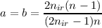
Given are term symbols (up to indices depending on actual case and group) and a and b coefficients. n is the number of electrons in an irrep with degeneracy nir. Note that not all cases are Roothaan cases.
All single electron cases are described by:
The 4d95s2 2D state of Ag, in symmetry I
All open shells are collected in a single open shell and
|
|
Example: The 4d55s1 7S state of Mo, treated in symmetry I
The two MOs must have different symmetries (not required for triplet coupling, see example 6.3.3). We have now two open shells and must specify three sets of (a,b), i.e. one for each pair of shells, following the keyword $rohf.
Example: CH2 in the 1B2 state from (3a1)1 (1b2)1, molecule in (x,z) plane.
This becomes tricky in general and we give only the most important case:
with parallel spin coupling of shells.
This covers e.g. the p5s1 3P states, or the d4s1 6D states of atoms. The coupling information is given following the keyword $rohf. The (a,b) within a shell are taken from above (6.3.2), the cross term (shell 1)–(shell 2) is in this case:
| a = | 1 always | ||
| b = | 2 ifn ≤ nir b =  ifn > nir ifn > nir |
Example 1: The 4d45s1 6D state of Nb, in symmetry I
Example 2: The 4d55s1 7S state of Mo, symmetry I (see Section 6.3.3) can also be done as follows.
The shells 5s and 4d have now been made inequivalent. Result is identical to 6.3.3 which is also more efficient.
Example 3: The 4d95s1 3D state of Ni, symmetry I
(see basis set catalogue, basis SV.3D requires this input and gives the energy you must get)
Valence states are defined as the weighted average of all CSFs arising from an electronic configuration (occupation): (MO)n. This is identical to the average energy of all Slater determinants.
 |
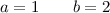
This covers, e.g. the cases n = 1 and n = 2nir - 1: p1, p5, d1, d9, etc, since there is only a single CSF which is identical to the average of configurations.
| n | = 2 | a | = 0 b = -nir | ||||
| n | = (2nir - 2) | a | =  | ||||
| b | =  |
| a | = 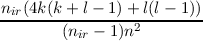 | ||
| b | = 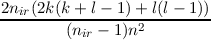 |
This covers most of the cases given above. A CSF results only if n = {1,(nir - 1), nir, (nir + 1), (2nir - 1)} since there is a single high-spin CSF in these cases.
The last equations for a and b can be rewritten in many ways, the probably most concise form is
| a | = 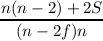 | ||
| b | =  . . |