Detailed description of methods implemented in the riper module is provided in Refs [107–111] and references therein. Here, only a short summary of the underlying theory is provided.
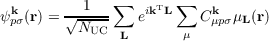
In periodic systems translational symmetry of solids leads to Bloch orbitals ψpσk and one-particle energies εpσk depending on the band index p, spin σ, and the wave vector k within the Brillouin zone (BZ), which is the unit cell of reciprocal space. The orbitals
|
| (7.1) |
are expanded in GTO basis functions μ(r -Rμ -L) ≡ μL(r) centered at atomic positions Rμ in direct lattice cells L over all NUC unit cells. This results in unrestricted Kohn-Sham equations
 | (7.2) |
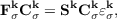
which may be solved separately for each k in the BZ. The same equations hold for the molecular case, where only L = k = 0 is a valid choice and NUC is one. Equation (7.2) contains the reciprocal space Kohn-Sham and the overlap matrices Fσk and Sk, respectively, obtained as Fourier transforms of real space matrices
| Fμνσk = ∑ LeikTLF μνσL S μνk = ∑ LeikTLS μνL. | (7.3) |
 | (7.4) |
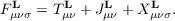
The total energy per unit cell E is calculated as the sum of the kinetic T, Coulomb J, and exchange-correlation EXC contributions,
 | (7.5) |
The key component of riper is a combination of RI approximation and CFMM applied for the
electronic Coulomb term [107,108,111]. In the RI scheme the total crystal electron density ρcryst is
approximated by an auxiliary crystal electron density  cryst
cryst
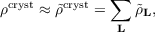 | (7.6) |
composed of unit cell auxiliary densities  L with
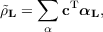 | (7.7) |
where αL denotes the vector of auxiliary basis functions translated by a direct lattice vector L.
The vector of expansion coefficients c is determined by minimizing the Coulomb repulsion D of the
residual density δρ = ρ -
 | (7.8) |
The RI approximation allows to replace four-center electron repulsion integrals (ERIs) by two- and three-center ones. In this formalism, elements JμνL of the Coulomb matrix are defined as
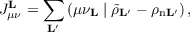 | (7.9) |
where ρn denotes the unit cell nuclear charge distribution. The total Coulomb energy including the nuclear contribution is
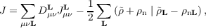 | (7.10) |
with the real space density matrix elements obtained by integration
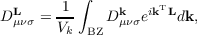 | (7.11) |
of the reciprocal space density matrix
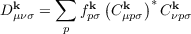 | (7.12) |
over the BZ with volume V k.
Equations (7.9) and (7.10) as well as other expressions appearing in the RI scheme require calculation of infinite lattice sums of the form
 | (7.13) |
where the distribution ρ1 in the central cell interacts with an infinite number of distributions ρ2L, i.e., ρ2 translated by all possible direct lattice vectors L. In the RI-CFMM scheme [107,108] the sum in Eq. (7.13) is partitioned into crystal far-field (CFF) and crystal near-field (CNF) parts. The CFF part contains summation over all direct space lattice vectors L for which the overlap between the distributions ρ1 and ρ2L is negligible. This part is very efficiently calculated using multipole expansions. The CNF contribution is evaluated using an octree based algorithm. In short, a cubic parent box enclosing all distribution centers of ρ1 and ρ2 is constructed that is large enough to yield a predefined number ntarg of distribution centers per lowest level box. The parent box is successively subdivided in half along all Cartesian axes yielding the octree. In the next step, all charge distributions comprising ρ1 and ρ2 are sorted into boxes based on their extents. Interactions between charges from well-separated boxes are calculated using a hierarchy of multipole expansions. Two boxes are considered well-separated if the distance between their centers is greater than sum of their lengths times 0.5×wsicl, where wsicl is a predefined parameter ≥ 2. The remaining contribution to the Coulomb term is obtained from direct integration. This approach results in nearly linear scaling of the computational effort with the system size.
The integral in Eq. (7.11) is evaluated approximately using a set of sampling points k. riper uses a Γ-point centered mesh of k points with weights wk, so that Eq. (7.11) can be written as
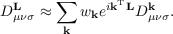 | (7.14) |
In 3D periodic systems each sampling point is defined by its components k1, k2 and k3 along the reciprocal lattice vectors b1, b2 and b3 as
 | (7.15) |
For 2D periodic systems k3 = 0. In case of 1D periodicity k3 = 0 and k2 = 0. In riper the three components kj (j = 1,2,3) of k are given as
 | (7.16) |
with nj (j = 1,2,3) as integer numbers. riper reduces the number of k points employed in actual calculation by a factor of two using time-inversion symmetry, i.e., the vectors k and -k are symmetry equivalent. The k point mesh can be specified providing the integer values nj within the data group $kpoints.
The number of k points required in a calculation critically depends on required accuracy. Generally, metallic systems require considerably more k points than insulators to reach the same precision. For metals, the number of k point also depends on parameters of the Gaussian smearing [112] used in riper. Please refer to Ref. [112] for more details.
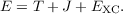
Achieving reasonable accuracy of DFT calculations for metals requires a higher number of k points than for semiconductors and insulators. The convergence with respect to the number of k points can be improved applying partial occupancies [112]. To achieve this, riper uses the Gaussian smearing method in which occupation numbers fnk are calculated as
![( ) ( [ ])
ϵnk --μ 1 ϵnk---μ-
fnk σ = 2 1- erf σ ,](DOK63x.png) | (7.17) |
where ϵnk are band (orbital) energies, μ is the Fermi energy and σ is the width of the smearing.
When smearing is applied the total energy E has to be replaced a generalized free energy F
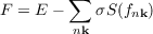 | (7.18) |
in order to obtain variational functional. riper output file reports the values of F as “FREE ENERGY” and the term -∑ nkσS(fnk) as “T*S”. In addition, the value of E for σ → 0 is given as “ENERGY (sigma->0)”.
Gaussian smearing can be switched on for riper calculations by simply providing the value of σ > 0 within the $riper data group using the keyword sigma, e.g., sigma 0.01. The value of σ should be as large as possible, but small enough to yield negligible value of the “T*S” term. Note, that the value of sigma has to be provided in atomic units. Please refer to Ref. [112] for a more detailed discussion.
The use of Gaussian smearing often requires much higher damping and orbital shifting. Please adjust the values for $scfdamp and $scforbitalshift if you encounter SCF convergence problems.
The optional keyword desnue can be used within the $riper data group to constrain the number of unpaired electrons. This can be used to force a certain multiplicity in case of an unrestricted calculation, e.g., desnue 0 for singlet and desnue 1 for dublet.
For calculations on very large molecular systems a low-memory modification of the RI approximation has been implemented within the riper module [110]. In the RI approximation minimization of the Coulomb repulsion of the residual density, Eq. (7.8), yields a system of linear equations
 | (7.19) |
where V is the Coulomb metric matrix with elements V αβ =  representing Coulomb
interaction between auxiliary basis functions and vector γ is defined as
representing Coulomb
interaction between auxiliary basis functions and vector γ is defined as
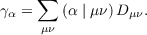 | (7.20) |
In the LMIDF approach a conjugate gradient (CG) iterative method is used for solution of Eq. (7.19). In order to decrease the number of CG iterations a preconditioning is employed, i.e., Eq. (7.19) is transformed using a preconditioner P to an equivalent problem
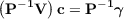 | (7.21) |
with an improved condition number resulting in faster convergence of the CG method. The iterative CG solver in riper employs one of the following preconditioners that are formed from blocks of the V matrix corresponding to the strongest and most important interactions between the auxiliary basis functions such that P-1V ≈I:
Pαβat = 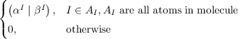 |
Pαβss =  |
Pαβsp = 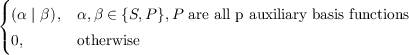 |
The costly matrix-vector products of the Vc type that need to be evaluated in each CG iteration
are not calculated directly. Instead, the linear scaling CFMM implementation presented
above is applied to carry out this multiplication since the elements of the Vc vector
represent Coulomb interaction between auxiliary basis functions α and an auxiliary density

 | (7.22) |
Hence, in contrast to conventional RI neither the V matrix nor its Cholesky factors need to be stored and thus significant memory savings are achieved.