10.2 Calculation of Excitation Energies

With the ricc2 program excitation energies can presently be calculated with the RI variants of the methods CCS/CIS, CIS(D), CIS(D_∞), ADC(2) and CC2. The CC2 excitation energies are obtained by standard coupled-cluster linear response theory as eigenvalues of the Jacobian, defined as derivative of the vector function with respect to the cluster amplitudes.

(10.8)

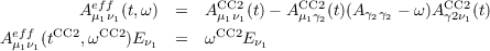
Since the CC2 Jacobian is a non-symmetric matrix, left and right eigenvectors are different and the right (left) eigenvectors E_νⁱ (E_μⁱ) are not orthogonal among themselves, but form a biorthonormal basis (if properly normalized):

(10.9)

To obtain excitation energies only the right or the left eigenvalue problem needs to be solved, but for the calculation of transition strengths and first-order properties both, left and right, eigenvectors are needed (see below). A second complication that arises from the non-symmetric eigenvalue problem is that in the case of close degeneracies within the same irreducible representation (symmetry) it can happen that instead of two close lying real roots a degenerate complex conjugated pair of excitation energies and eigenvectors is obtained. CC2 (and also other standard coupled-cluster response methods) are thus not suited for the description of conical intersections etc. For the general theory behind coupled cluster response calculations see e.g. ref.  [151,152] or other reviews.

The ricc2 program exploits that the doubles/doubles block of the CC2 Jacobian is diagonal and the (linear) eigenvalue problem in the singles and doubles space can be reformulated as a (non-linear) eigenvalue problem in single-substitution space only:

The solution of the CC2 eigenvalue problem can be started from the solutions of the CCS eigenvalue problem (see below) or the trial vectors or solutions of a previous CC2 excitation energy calculation. The operation count per transformed trial vector for one iteration for the CC2 eigenvalue problem is about 1.3–1.7 times the operation count for one iteration for the cluster equations in the ground-state calculation—depending on the number of vectors transformed simultaneously. The disk space requirements are about O(V + N)N_x double precision words per vector in addition to the disk space required for the ground state calculation.

CCS excitation energies are obtained by the same approach, but here double-substitutions are excluded from the expansion of the excitation or eigenvectors and the ground-state amplitudes are zero. Therefore the CCS Jacobian,

(10.10)

is a symmetric matrix and left and right eigenvectors are identical and form an orthonormal basis. The configuration interaction singles (CIS) excitation energies are identical to the CCS excitation energies. The operation count for a RI-CIS calculation is (ON²N_x) per iteration and transformed trial vector.

The second-order perturbative correction CIS(D) to the CIS excitation energies is calculated from the expression

(10.11)

(Note that t^MP1 are the first-order double-substitution amplitudes from which also the MP2 ground-state energy is calculated; the first-order single-substitution amplitudes vanish for a Hartree–Fock reference due to the Brillouin theorem.) The operation count for a RI-CIS(D) calculation is similar to that of a single iteration for the CC2 eigenvalue problem. Also disk space requirements are similar.

Running excitation energy calculations: The calculation of excitation energies is initiated by the data group $excitations in which at least the symmetries (irreducible representations) and the number of the excited states must be given (for other options see Section 20.2.19). With the following input the ricc2 program will calculate the lowest two roots (states) for the symmetries A₁ and B₁ of singlet multiplicity ^* at the CIS, CIS(D) and CC2 level with default convergence thresholds. Ground-state calculations will be carried out for MP2 (needed for the CIS(D) model and used as start guess for CC2) and CC2.

The single-substitution parts of the right eigenvectors are stored in files named CCRE0-s--m-xxx, where s is the number of the symmetry class (irreducible representation), m is the multiplicity, and xxx the number of the excitation within the symmetry class. For the left eigenvectors the single-substitution parts are stored in files named CCLE0-s--m-xxx. These files can be kept for later restarts.

Trouble shooting: For the iterative second-order methods CIS(D_∞), ADC(2), and CC2 the solution of the nonlinear partitioned eigenvalue problem proceeds usually in three steps:

1.

solution of the CCS/CIS eigenvalue problem to generate reasonable start vectors; the eigenvectors are converged in this step only to a remaining residual norm < preopt

2.

pre-optimization of the eigenvectors by a robust modified Davidson algorithm (see ref.  [8]) using the LINEAR CC RESPONSE SOLVER until the norm of all residuals are below preopt, combined with a DIIS extrapolation for roots assumed to be converged below the threshold thrdiis.

3.

solution of the nonlinear eigenvalue problem with a DIIS algorithm using the DIIS CC RESPONSE SOLVER until the norm of the residuals are below the required threshold conv

This procedure is usually fairly stable and efficient with the default values for the thresholds. But for difficult cases it can be necessary to select tighter thresholds. In case of convergence problems the first thing do is to verify that the ground state is not a multireference case by checking the D1 diagnostic. If this is not the case the following situations can cause problems in the calculation of excitation energies:

• almost degenerate roots in the same symmetry class
• complex roots (break down of the CC approximation close to conical intersections)
• large contributions from double excitations

The first two reasons can be identified by running the program with a print level ≤ 3. It will then print in each iteration the actual estimates for the eigenvalues. If some of these are very close or if complex roots appear, you should make sure that the DIIS procedure is not switched on before the residuals of the eigenvectors are small compared to the differences in the eigenvalues. For this, thrdiis (controlling the DIIS extrapolation in the linear solver) should be set about one order of magnitude smaller than the smallest difference between two eigenvalues and preopt (controlling the switch to the DIIS solver) again about one order of magnitude smaller then thrdiis.

Tighter thresholds or difficult situations can make it necessary to increase the limit for the number of iterations maxiter.

In rare cases complex roots might persist even with tight convergence thresholds. This can happen for CC2 and CIS(D_∞) close to conical intersections between two states of the same symmetry, where CC response can fail due to its non-symmetric Jacobian. In this case one can try to use instead the ADC(2) model. But the nonlinear partitioned form of the eigenvalue problem used in the ricc2 program is not well suited to deal with such situations.

Diagnostics for double excitations: As pointed out in ref.  [10], the %T₁ diagnostic (or %T₂ = 100 - %T₁) which is evaluated directly from the squared norm of the single and double excitation part of the eigenvectors %T₁ = 100 ⋅ T₁∕(T₁ + T₂) with T_i = ∑ _μiE_μi² where the excitation amplitudes are for spin-free calculations in a correspoding spin-adapted basis (which is not necessarily normalized) has the disadvantage that the results depend on the parameterization of the (spin-adapted) excitation operators. This prevents in particular a simple comparison of the results for singlet and triplet excited states if the calculations are carried out in a spin-free basis. With the biorthogonal representation for singlet spin-coupled double excitations [151] results for %T₁ also differ largely between the left and right eigenvectors and are not invariant with respect to unitary transformations of the occupied or the virtual orbitals.

The ricc2 module therefore uses since release 6.5 an alternative double excitation diagnostic, which is defined by %₁ = 100 *₁∕(₁ + ₂) with ₁ = ∑ _aiE_ai² and ₂ = ∑ _i>j ∑ _a>bE_aibj² with E_ai and E_aibj in the spin-orbital basis. They are printed in the summaries for excitation energies under the headings %t1 and %t2. For spin-adapted excitation amplitudes ₁ and ₂ have to be computed from respective linear combinations for the amplitudes which reproduce the values in the spin-orbital basis. For ADC(2), which has a symmetric secular matrix with identical left and right normalized eigenvectors ₁ and ₂ are identical with the contributions from the singles and doubles parts for the eigenvectors to the trace of the occupied or virtual block of the (orbital unrelaxed) difference density between the ground and the excited state, i.e. the criterium proposed in ref.  [10]. Compared to the suggestion from ref.  [10] ₁ and ₂ have the additional advantage of that they are for all methods guaranteed to be postive and can be evaluated with the same insignificantly low costs as T₁ and T₂. They are invariant with respect to unitary transformations of the occupied or the virtual orbitals and give by construction identical results in spin-orbital and spin-free calculations. For CC2 and CIS(D_∞) the diagnostics ₁ and ₂ agree for left and right eigenvectors usually with a few 0.01%, for CIS(D) and ADC(2) they are exactly identical. For singlet excitations in spin-free calculations, %₂ is typically by a factors of 1.5–2 larger than %T₂. The second-order methods CC2, ADC(2), CIS(D_∞) and CIS(D) can usually be trusted for %₂ ≤ 15%.

For compatibility, the program can be switched to use of the old %₁ and %₂ diagnostics (printed with the headers ||T1|| and ||T2||) by setting the flag oldnorm in the data group $excitations. Note that the choice of the norm effects the individual results left and right one- and two-photon transition moments, while transition strengths and all other observable properties independent of the individual normalization of the right and left eigenvectors.

The %₂ and %T₂ diagnostics can not be monitored in the output of the (quasi-) linear solver. But it is possible to do in advance a CIS(D) calculation. The CIS(D) results for the %₂ and %T₂ correlate usually well with the results for this diagnostic from the iterativ second-order models, as long as there is clear correspondence between the singles parts of the eigenvectors. Else the DIIS solver will print the doubles diagnostics in each iteration if the print level is set > 3. States with large double excitation contributions converge notoriously slow (a consequence of the partitioned formulation used in the ricc2 program). However, the results obtained with second-order methods for doubly excited states will anyway be poor. It is strongly recommended to use in such situations a higher-level method.

Visualization of excitations: An easy way to visualize single excitations is to plot the natural transition orbitals that can be obtained from a singular value decomposition of the excitation amplitudes. See Sec. 18.1.6 for further details.

Another, but computational more involved possibility is plot the difference density between the ground and the respective excited state. This requires, however, a first-order property or gradient calculation for the excited state to obtain the difference density. For further details see Sec. 10.3.3.