Transition moments (for one-photon transitions) are presently implemented for excitations out of the ground state and for excitations between excited states for the coupled cluster models CCS and CC2. Transition moments for excitations from the ground to an excited state are also available for ADC(2), but use an additional approximation (see below). Note, that for transition moments (as for excited-state first-order properties) CCS is not equivalent to CIS and CIS transition moments are not implemented in the ricc2 program.
Two-photon transition moments are only available for CC2.
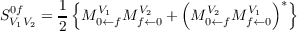
In response theory, transition strengths (and moments) for transitions from the ground to excited state are identified from the first residues of the response functions. Due to the non-variational structure of coupled cluster different expressions are obtained for the CCS and CC2 “left” and “right” transitions moments M0←fV and Mf←0V . The transition strengths SV 1V 20f are obtained as a symmetrized combinations of both [154]:
|
| (10.21) |
Note, that only the transition strengths SV 1V 20f are a well-defined observables but not the transition moments M0←fV and Mf←0V . For a review of the theory see refs. [152,154]. The transition strengths calculated by coupled-cluster response theory according to Eq. (10.21) have the same symmetry with respect to an interchange of the operators V 1 and V 2 and with respect to complex conjugation as the exact transition moments. In difference to SCF (RPA), (TD)DFT, or FCI, transition strengths calculated by the coupled-cluster response models CCS, CC2, etc. do not become gauge-independent in the limit of a complete basis set, i.e., for example the dipole oscillator strength calculated in the length, velocity or acceleration gauge remain different until also the full coupled-cluster (equivalent to the full CI) limit is reached.
For a description of the implementation in the ricc2 program see refs. [11,150]. The calculation of transition moments for excitations out of the ground state resembles the calculation of first-order properties for excited states: In addition to the left and right eigenvectors, a set of transition Lagrangian multipliers μ has to be determined and some transition density matrices have to be constructed. Disk space, core memory and CPU time requirements are thus also similar.
The single-substitution parts of the transition Lagrangian multipliers μ are saved in files named CCME0-s--m-xxx.
To obtain the transition strengths for excitations out of the ground state the keyword spectrum must be added with appropriate options (see Section 20.2.19) to the data group $excitations; else the input is same as for the calculation of excitation energies and first-order properties:
For the ADC(2) model, which is derived by a perturbation expansion of the expressions for exact
states, the calculation of transition moments for excitations from the ground to an excited state
would require the second-order double excitation amplitudes for the ground state wavefunction,
which would lead to operation counts scaling as  (
( 6), if no further approximations are
introduced. On the other hand the second-order contributions to the transition moments are
usually not expected to be important. Therefore, the implementation in the ricc2 program
neglects in the calculation of the ground to excited state transition moments the contributions
which are second order in ground state amplitudes (i.e. contain second-order amplitudes or
products of first-order amplitudes). With this approximation the ADC(2) transition moments are
only correct to first-order, i.e. to the same order to which also the CC2 transition moments
are correct, and are typically similar to the CC2 results. The computational costs for
the ADC(2) transition moments are (within this approximation) much lower than for
CC2 since the left and right eigenvectors are identical and no lagrangian multipliers
need to be determined. The extra costs (i.e. CPU and wall time) for the calculations
of the transitions moments are similar to the those for two or three iterations of the
eigenvalue problem, which reduces the total CPU and wall time for the calculation
of a spectrum (i.e. excitation energies and transition moments) by almost a factor of
three.
6), if no further approximations are
introduced. On the other hand the second-order contributions to the transition moments are
usually not expected to be important. Therefore, the implementation in the ricc2 program
neglects in the calculation of the ground to excited state transition moments the contributions
which are second order in ground state amplitudes (i.e. contain second-order amplitudes or
products of first-order amplitudes). With this approximation the ADC(2) transition moments are
only correct to first-order, i.e. to the same order to which also the CC2 transition moments
are correct, and are typically similar to the CC2 results. The computational costs for
the ADC(2) transition moments are (within this approximation) much lower than for
CC2 since the left and right eigenvectors are identical and no lagrangian multipliers
need to be determined. The extra costs (i.e. CPU and wall time) for the calculations
of the transitions moments are similar to the those for two or three iterations of the
eigenvalue problem, which reduces the total CPU and wall time for the calculation
of a spectrum (i.e. excitation energies and transition moments) by almost a factor of
three.
For the calculation of transition moments between excited states a set of Lagrangian multipliers μ has to be determined instead of the μ for the ground state transition moments. From these Lagrangian multipliers and the left and right eigenvectors one obtaines the “right” transition moment between two excited states i and f as
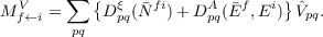 | (10.22) |
where  are the matrix elements of the perturbing operator. A similar expression is obtained for
the “left” transition moments. The “left” and “right” transition moments are then combined to
yield the transition strength
are the matrix elements of the perturbing operator. A similar expression is obtained for
the “left” transition moments. The “left” and “right” transition moments are then combined to
yield the transition strength
 | (10.23) |
As for the ground state transitions, only the transition strengths SV 1V 2if are a well-defined observables but not the transition moments Mi←fV and Mf←iV .
The single-substitution parts of the transition Lagrangian multipliers μ are saved in files named CCNE0-s--m-xxx.
To obtain the transition strengths for excitations between excited states the keyword tmexc must be added to the data group $excitations. Additionally, the initial and final states must be given in the same line; else the input is same as for the calculation of excitation energies and first-order properties:
For closed-shell restricted and high-spin open-shell unrestricted Hartree-Fock reference states two-photon transition moments for one-electron operators can be computed at the CCS and the CC2 level. The implementation is restricted to real abelian point groups (D2h and its subgroups) and for CC2 without spin-component scaling. The response theory for the calculation of two-photon transition moments with coupled cluster methods has been described in [155,156], the RI-CC2 implementation in [157].
Similar as for one-photon transitions also for two-photon transitions the non-variational structure of coupled cluster theory leads to different expressions for “left” and “right” transition moments M0←fV 1V 2 and Mf←0V 3V 4. Only the transition strengths SV 1V 2,V 3V 40f which are obtained as symmetrized combination of both [154,156],
 | (10.24) |
is an observable quantity.
The ricc2 program prints in the output in addition to the transition moments in atomic units also the rotationally averaged transition strengths in atomic units and transition rates in Göppert-Maier (GM) units for linear, perpendicular and circular polarized beams.
In addition to the input for the excitation energies, the computation of two-photon transition moments requires the keyword twophoton in the data group $excitations and the data group for the numerical Laplace transformation $laplace.
The syntax for the input for states is the same as for one-photon transition moments (option spectrum). Frequencies ω2 for the photon associated in the “right” transition moment, Mf←0V 1V 2(ω2), with the second operator in each operator pair can be given in atomic units with the suboption freq. It corresponds to the frequency ω in Eq. 10.24. The frequency associated with the first operator is automatically determined from the sum rule ω1 = ω0f -ω2, where ω0f is the frequency for the transition f ← 0. The “left” transition moments M0←fV 1V 2 are computed for the frequencies with the opposite sign. If not specified, the two-photon transition moments are computed for the case that both photons have the same frequency, i.e. their energies are set for each state to 1/2 of the transition energy, which is the most common case.
For the calculation of oscillator strengths for triplet excited states and phosphorescence lifetimes for molecules without heavy atoms the ricc2 program provides as alternative to the relativistic two-component variant a perturbative SOC-PT-CC2 approach which works with one-component wavefunctions. In SOC-PT-CC2 the oscillator strengths for triplet excited states are calculated as first derivatives of the (spin-forbidden) oscillator strengths for one-component wavefunctions with respect to the strength of the spin-orbit coupling (SOC) in the limit of zero spin-orbit coupling. The spin-orbit coupling is treated within the effictive spin-orbit mean field approximation, where the mean field two-electron contribution is computed from the Hartree-Fock density. The SOC-PT-CC2 approach is about an order of magnitude faster than the computation of oscillator strengths with the two-component RI-CC2 variant. Scalar relativistic effects from the spin-free X2C Hamiltonian can be included by using the spin-free X2C Hamiltonian for the Hartree-Fock reference wavefunction. The theory and the implementation are described in [158].
The implementation is restricted to closed-shell Hartree-Fock reference wavefunctions and CC2 without spin-component scaling. For carrying out such calculations one needs in addition to the input for the excitation energies for triplet states the keyword momdrv and the data group for the numerical Laplace transformation $laplace.
For phosphorescence lifetimes the frequency has to be set to zero with the option freq=0.0d0 and the operator pair has to be set to (diplen,soc) for the dipole operator and the SOC operator in the SOMF approximation, so that the input frequency 0.0d0 is associated with the SOC operator and the ground to excited state transition frequency ω0f with the dipole operator.
The program prints in the output in addition to the first-order induced transition moments for the operator pair (diplen,soc) the induced oscillator strengths and the life times.