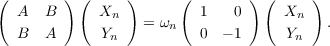
The Bethe–Salpeter (BS) excitation energies ωn are obtained as solutions of a pseudo-Hermitian eigenvalue equation, which has the same form as in time-dependent Hartree–Fock (TD-HF) theory. For the sake of simplicity, only the equations for singlet excitation energies based on a closed-shell reference are given below. The orbitals are assumed to be real.
|
| (13.7) |
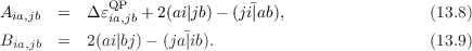
In the following, the indices a,b,… (i,j,…) refer to unoccupied (doubly occupied) spatial orbitals, the indices p,q,r,… include both doubly and unoccupied orbitals. The definitions of the matrices A and B differ in the one-particle energies, which are the orbital energies in case of TD-HF and the GW quasi-particle energies εQP in case of BS. Also, the exchange interaction is screened in case of BS,
 | (13.10) |
is screened by the inverse of the dielectric function,
![ϵ = δ δ - 2(pq|rs)[χ (ω = 0)] , (13.11)
pq,rs prqs ∑ 0 rs,rs
[χ0(ω = 0)] = δraδsi +-δriδsa, (13.12)
rs,rs ia εQiP - εQaP](DOK222x.png)
 | (13.13) |
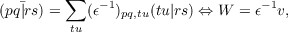
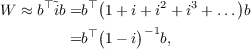
To obtain W, the RI-approximation is introduced for the two-electron integrals. As a direct result, the inversion ϵ is replaced by the inversion of a matrix in the auxiliary basis:
 | (13.14) |
 | (13.15) |
For further details, we refer to Ref. [178].
The BSE method is implemented in the escf module. It is activated by the keyword $bse. Its features and different variants are discussed in the following.
The BSE method supports both Hartree–Fock and Kohn–Sham references, that is, orbitals obtained from a dscf or ridft computation. Note that symmetry is only supported up to D2h and its subgroups. In case of wave functions of higher symmetry, the orbitals have to be converted using define’s option susy to a subgroup of D2h.
Singlet, triplet and spin-unrestricted excitation energies based on the Bethe–Salpeter equation are available in escf. Similar to the RPA and TDA variants in TD-HF, the eigenvalues of the full 2 × 2 “super-matrix” can be computed, or of A only. To define these options, the same input blocks as for a TD-HF computation are read in: $scfinstab and $soes. See Section 8 for details.
The BSE method reads in quasi-particle energies obtained from a preceding GW calculation. It supports all different GW methods available in escf. Note that if orbitals are excluded from excitations by the flag $freeze, the same number of occupied orbitals have to be frozen in the GW and BSE calculations.
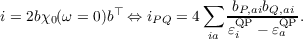
By default, the matrices A and W are set up using quasi-particle energies. To set up A using KS/HF orbital energies instead, i.e.
 | (13.16) |
the option noqpa has to be added to the $bse block in control. Similarly, if the denominator in χ0 and, consequently, the static screened interaction should be constructed using KS/HF orbital energies instead of GW quasi-particle energies, the option noqpw has to be set. The quasi-particle energies are read in from the file qpenergies.dat, which has to be created in a preceding GW calculation using escf. A different file name can be defined using the option file in the $bse block.
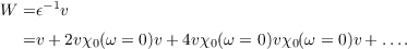
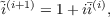
The static screened interaction is obtained from the auxiliary matrix ĩ. By default, this is computed by Cholesky decomposition and inversion of (1 - i)-1. An alternative iterative procedure,
 | (13.17) |
is activated by the option iterative. The convergence threshold (default: 1.0d-12) and maximum number of iterations (default: 100) can be adjusted by the options thrconv and iterlim, respectively.
The static screened interaction is computed using the RI approximation, therefore, an auxiliary basis set is required. Since the integrals are similar to those in MP2, the cbas auxiliary basis sets are recommended. They can be conveniently defined using the cc sub-menu of define.