Treatment of Solvation Effects with Cosmo

17.2 Treatment of Solvation Effects with COSMO

The Conductor-like Screening Model [184] (COSMO) is a continuum solvation model (CSM), where the solute molecule forms a cavity within the dielectric continuum of permittivity ε that represents the solvent. The charge distribution of the solute polarizes the dielectric medium. The response of the medium is described by the generation of screening charges on the cavity surface.

CSMs usually require the solution of the rather complicated boundary conditions for a dielectric in order to obtain the screening charges. COSMO instead uses the much simpler boundary condition of vanishing electrostatic potential for a conductor,

tot Φ = 0.

This represents an electrostatically ideal solvent with ε = ∞. The vector of the total electrostatic potential on the cavity surface segments is determined by the solute potential Φ^sol, which consist of the electronic and the nuclear part, and the vector of the screening charges q,

tot sol Φ = Φ +Aq = 0.

A is the Coulomb matrix of the screening charge interactions. For a conductor, the boundary condition Φ^tot = 0 defines the screening charges as

-1 sol q = - A Φ .

To take into account the finite permittivity of real solvents, the screening charges are scaled by a factor.

ε--1- f(ε) = ε+ 1 q⋆ = f(ε)2q

The deviation between the COSMO approximation and the exact solution is rather small. For strong dielectrics like water it is less than 1%, while for non-polar solvents with ε ≈ 2 it may reach 10% of the total screening effects. However, for weak dielectrics, screening effects are small and the absolute error therefore typically amounts to less than one kcal/mol. As shown in [185] ions can be described more accurately by using the scaling factor f(ε) = ε-ε+10

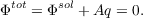
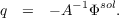
. This also leads to results (e.g. by comparing solvation free energies) more or less identical to IEFPCM or SS(V)PE. This is possible since TURBOMOLE version 7.1 by adding the keyword ions to the epsilon option in the $cosmo section (see 20.2.10).

The dielectric energy, i.e. the free electrostatic energy gained by the solvation process, is half of the solute-solvent interaction energy.

1 † sol Ediel = 2f (ε)q Φ

The total free energy of the solvated molecule is the sum of the energy of the isolated system calculated with the solvated wave function and the dielectric energy

E = E(Ψsolv)+ Ediel.

A COSMO energy calculation starts with the construction of the cavity surface grid. Within the SCF procedure, the screening charges are calculated in every cycle and the potential generated by these charges is included into the Hamiltonian. This ensures a variational optimization of both the molecular orbitals and the screening charges and allows for the evaluation of analytic gradients.

Radii based Cavity Construction: In order to ensure a sufficiently accurate and efficient segmentation of the molecular shaped cavity the COSMO implementation uses a double grid approach and segments of hexagonal, pentagonal, and triangular shape. The cavity construction starts with a union of spheres of radii R_i + RSOLV for all atoms i. In order to avoid problems with symmetric species, the cavity construction uses de-symmetrized coordinates. The coordinates are slightly distorted with a co-sinus function of amplitude AMPRAN and a phase shift PHSRAN. Initially a basis grid with NPPA segments per atom is projected onto atomic spheres of radii R_i + RSOLV . In order to avoid the generation of points in the problematic intersections, all remaining points, which are not in the interior of another sphere, are projected downwards onto the radius R_i. In the next step a segment grid of NSPH segments per H atom and NSPA segments for the other atoms is projected onto the surface defined by R_i. The basis grid points are associated to the nearest segment grid centers and the segment coordinates are re-defined as the center of area of their associated basis grid points, while the segment area is the sum of the basis grid areas. Segments without basis grid points are discarded. In order to ensure nearest neighbor association for the new centers, this procedure is repeated once. At the end of the cavity construction the intersection seams of the spheres are paved with individual segments, which do not hold associated basis grid points.

Density based Cavity Construction: Instead of using atom specific radii the cavity can be defined by the electron density. In such an isodensity cavity construction one can use the same density value for all atoms types or the so-called scaled isodensity values. In the later approach different densities are used for the different atom types. The algorithm implemented in TURBOMOLE uses a marching tetrahedron algorithm for the density based cavity construction. In order to assure a smooth density change in the intersection seams of atoms with different isodensity specification, this areas are smoothened by a radii based procedure.

A-Matrix Setup: The A matrix elements are calculated as the sum of the contributions of the associated basis grid points of the segments k and l if their distance is below a certain threshold, the centers of the segments are used otherwise. For all segments that do not have associated basis grid points, i.e. intersection seam segments, the segment centers are used. The diagonal elements A_kk that represent the self-energy of the segment are calculated via the basis grid points contributions, or by using the segment area A_kk ≈ 3.8 √ --
ak , if no associated basis grid points exist.

Outlying charge correction: The part of the electron density reaching outside the cavity causes an inconsistency that can be compensated by the "outlying charge correction". This correction will be performed at the end of a converged SCF or an iterative MP2 calculation and uses an outer surface for the estimation of the energy and charge correction [186]. The outer surface is constructed by an outward projection of the spherical part of the surface onto the radius R_i + ROUTF *RSOLV . It is recommended to use the corrected values.

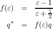
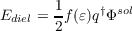
Numerical Frequency Calculation: The calculation of harmonic frequencies raises the problem of non-equilibrium solvation in the COSMO framework, because the molecular vibrations are on a time scale that do not allow a re-orientation of the solvent molecules. Therefore, the total response of the continuum is split into a fast contribution, described by the electronic polarization, and a slow term related to the orientational relaxation. As can be shown [187] the dielectric energy for the disturbed state can be written as

d 1 0 0 1 2 Δ Δ 0 Δ Ediel = 2f(ε)q(P )Φ (P )+ 2f(n )q(P )Φ(P )+ f(ε)q(P )Φ (P ),

where P^Δ denotes the density difference between the distorted state and the initial state with density P⁰. The interaction is composed of three contributions: the initial state dielectric energy, the interaction of the potential difference with the initial state charges, and the electronic screening energy that results from the density difference. The energy expression can be used to derive the correspondent gradients, which can be applied in a numerical frequency calculation. Because the COSMO cavity changes for every distorted geometry the initial state potential has to be mapped onto the new cavity in every step. The mapped potential of a segment of the new cavity is calculated from the distance-weighted potentials of all segments of the old cavity that fulfill a certain distance criterion. The mapped initial state screening charges are re-calculated from the new potential.

Iterative MP2 COSMO: For ab initio MP2 calculations within the CSM framework three alternatives can be found in the literature [188]. The first approach, often referred to as PTE, performs a normal MP2 energy calculation on the solvated HF wave function. The response of the solvent, also called reaction field, is still on the HF level. It is the only of the three approaches that is formally consistent in the sense of second-order perturbation theory [189,190]. In the so-called PTD approach the vacuum MP2 density is used to calculate the reaction field. The third approach, often called PTED, is iterative so that the reaction field reflects the density of the first-order wave function. In contrast to the PTE approach the reaction field, i.e. the screening charges, change during the iterations until self consistency is reached. Gradients are available on the formally consistent PTE level only [191].

Vertical excitations and Polarizabilities for TDDFT, TDA and RPA: The escf program accounts for the COSMO contribution to the excitation energies and polarizabilities. The COSMO settings have to be defined for the underlying COSMO dscf or ridft calculation. In case of the excitation energies the solvent response will be divided into the so-called slow and fast term [187,192]. The screening function of the fast term depends on the refractive index of the solvent which can be defined in the input. If only the COSMO influence on the ground state should be taken into account we recommend to perform a normal COSMO calculation (dscf or ridft) and to switch off COSMO (i.e. deactivate $cosmo) before the escf calculation.

The Direct COSMO-RS method (DCOSMO-RS): In order to go beyond the pure electrostatic model a self consistent implementation of the COSMO-RS model the so-called "Direct COSMO-RS" (DCOSMO-RS) [193] has been implemented in ridft and dscf.

COSMO-RS (COSMO for Real Solvents) [194,195] is a predictive method for the calculation of thermodynamic properties of fluids that uses a statistical thermodynamics approach based on the results of COSMO SCF calculations for molecules embedded in an electric conductor, i.e. using f(ε) = 1. The liquid can be imagined as a dense packing of molecules in the perfect conductor (the reference state). For the statistical thermodynamic procedure this system is broken down to an ensemble of pair wise interacting surface segments. The interactions can be expressed in terms of surface descriptors. e.g. the screening charge per segment area (σ_t = q_t∕a_t). Using the information about the surface polarity σ and the interaction energy functional, one can obtain the so-called σ-potential (μ_S(σ;T)). This function gives a measure for the affinity of the system S to a surface of polarity σ. The system S might be a mixture or a pure solvent at a given temperature T. Because the parabolic part of the potential can be described well by the COSMO model, we subtract this portion form the COSMO-RS potential:

˜μS(σ;T) = μS(σ;T)- (1- f(ε))c0σ2.

The parameter c₀ can be obtained from the curvature of a COSMO-RS σ-potential of a nonpolar substance, e.g. hexane. Thus, the remaining part of the chemical potential of a compound i with mole fraction x_i in the mixture Si can be expressed as:

m μi ~= ∑ f a ˜μ (σ;T) +μi + kT ln(x). t=1 polt S C,S i

where the combinatorial term μ_C,Sⁱ accounts for effects due to the size and shape differences of the molecules in the mixture and a_t denotes the area of segment t. The kT ln(x_i) can be skipped for infinite dilution. The factor f_pol has been introduced to account for the missing solute-solvent back polarization. The default value is one in the current implementation. The free energy gained by the solvation process in the DCOSMO-RS framework is the sum of the dielectric energy of the COSMO model and the chemical potential described above:

Ediel,RS = 1f (ε)q†Φsol + μi = Ediel + μi 2

From the above expression the solvent operator

^RS can be derived by functional derivative with respect to the electron density:

RS ∑m f(ε)qt +-qtΔRS cos ∑m -qΔtRS- ˆV = - |rt - r| = ˆV - |rt - r|. t=1 t=1

Thus, the solvation influence of the COSMO-RS model can be viewed as a correction of the COSMO screening charges q_t. The additional charges denoted as q_t^ΔRS can be obtained from q^ΔRS = -A^-1Φ^ΔRS, where the potential Φ^ΔRS arises from the chemical potential of the solute in the solvent:

ΔRS ( δ˜μS) ϕt = at δq-- . q=qt

In order to get a simple and differentiable representation of the COSMO-RS σ-potential μ_S(σ;T), we use equally spaced cubic splines. An approximate gradient of the method has been implemented. DCOSMO-RS can be used in SCF energy and gradient calculations (geometry optimizations) with dscf, ridft, grad, and rdgrad. Please regard the restriction of the DCOSMO-RS energy explained in the keyword section 20.2.10. Because the DCOSMO-RS contribution can be considered as a slow term contribution in vertical excitations it does not have to be taken into account in response calculations. For the calculation of vertical excitation energies it is recommended to use the mos of a DCOSMO-RS calculation in a COSMO response calculation (see above).

Solvation effects on excited states using COSMO in ricc2: The COSMO approach has been recently implemented into the ricc2 module of TURBOMOLE. It is now possible to equilibrate the solvent charges for any excited state or the ground state as mentioned in the MP2 section above. Using the methods CCS/CIS or ADC(2) the implementation is complete, for CC2 or higher methods, however it still has to be proven if there are terms missing The recent implementation contains contributions to the off-diagonal elements of the one-electron density. Furthermore the energy contributions for non-equilibrated states can be calculated. Non-equilibrated means in this sense, that the slow part of the solvent charges (described by f(ε)) are still equilibrated with a given initial state, while the fast electronic part of the solvent charges (described by f(n²)) are in equilibrium with the target state. To handle this one has to do a macro iteration, like in MP2. This macro iteration can be managed with the script ’cc2cosmo’ which is the same as ’mp2cosmo’ but using ricc2 instead of rimp2 or mpgrad. To set up the basic settings one can reuse the cosmoprep module, note that one has to specify the refractive index ’refind’ when observing excited states. To specify the state to which the solvent charges should be equilibrated one inserts the keyword ’cosmorel state=(x)’, where the ground state (x) is used normally but can be replaced by any requested excited state. Make sure to request relaxed properties for any desired state, otherwise the COSMO macro iteration will not work in ricc2. The off-diagonal contributions mentioned above can be switched off by setting the keyword ’nofast’ in $cosmo. A typical input might look like:

$ricc2
  adc(2)
$excitations
  irrep=a’  multiplicity=  1  nexc=  1  npre=  1  nstart=  1
  irrep=a"  multiplicity=  1  nexc=  1  npre=  1  nstart=  1
  exprop relaxed states=all
$response
  fop relaxed
$cosmo
  epsilon=   50.000
  rsolv= 1.30
  refind=   3.0000
  cosmorel state=(a" 1)
# nofast
$cosmo_correlated
$cosmo_atoms
...

This would deliver an excited state calculation for the lowest singlet A’ and A" excitations using the ADC(2) method. The solvent charges are equilibrated to state 1¹A" and the non-equilibrium energy contributions for the MP2 ground state and the 1¹A’ excited state are calculated furthermore. All contributions to the one-electron density are included since the proper keyword is commented out. Note: when doing solvent relaxations with the CCS/CIS model, no request of relaxed ground–state properties are needed, since the relaxed ground state is identical to the HF ground state. A short summary of the COSMO input is given at the beginning of the ricc2 output as well as a summary of the energy contributions is given at the end of the ricc2 output.

[next] [prev] [prev-tail] [front] [up]