Molecular properties (electrostatic moments, relativistic corrections, population analyses for densities and MOs, construction of localized MOs, NTOs, etc.) can be calculated with proper. This program is menu-driven and reads the input that determines which properties are evaluated from standard input (i.e. the terminal or an input file if started as proper < inputfile). The control file and files referenced therein are only used to determine the molecular structure, basis sets, and molecular orbitals and to read results computed before with other programs.
proper is a post-processing tool, mainly intended for an interactive use. Several functionalities are also integrated in the programs that generate MOs or densities and can be invoked directly from the modules dscf, ridft, rimp2, mpgrad, ricc2 and egrad, if corresponding keywords are set in the control file. If one wants to skip the MO- or density generating step for dscf, ridft, rimp2, mpgrad, ricc2 it is possible to directly jump to the routine that carries out the analyses by starting the program with "<program> -proper". (For ricc2 it is, however, recommended to use instead ricctools -proper.) Currently, the respective keywords have to be inserted by hand (not with define) in the control file.
Here we briefly present the functionalities. A detailed description of the keywords that can be used in combination with the -proper flag is found Section 20.2.25.
The proper program tries on start to read all densities that have been pre-calculated with any of the other programs of the TURBOMOLE package, prints a list with the densities that have been found and selects one of them for the calculation of properties. The default choice can be changed in the menu that is entered with the option dens. Here one can also list or edit additional attributes of the densities or build linear combinations of the available densities to form differences and superposition of densities.
The feature can thus be used to evaluate difference densities between the ground and excited electronic states or differences between densities calculated with different electronic structure methods.
The selected density can then be used in the subsequent menues to evaluate a variety of properties as expectation values or on a grid of points to generate interface files for visualization.
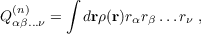
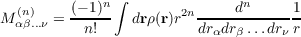
Use the mtps option in the eval menu in proper, or add the $moments keyword control file when you start a program with the -proper flag to evaluate electrostatic moments. Up to quadrupole moments are calculated by default, on request also octupole moments are available. By default unnormalized traced cartesian moments are calculated which are defined as
The option relcor in the eval menu of proper or the keyword $mvd (when starting a program with the -proper flag) initiate the calculation of relativistic corrections. With the -proper flag they are calculated for the SCF or DFT total density in case of dscf and ridft, for the SCF+MP2 density in case of rimp2 and mpgrad and for that of the calculated excited state in case of egrad. Quantities calculated are the expectation values ⟨p2⟩ , ⟨p4⟩ and the Darwin term ⟨∑ A1∕ZA * ρ(RA)⟩. Note, that at least the Darwin term requires an accurate description of the cusp in the wave function, thus the use of basis sets with uncontracted steep basis functions is recommended. Moreover note, that the results for these quantities are not really reasonable if ECPs are used (a respective warning is written to the output).
For population analyses enter the pop menu of proper. The available options and parameters that can be specified are the same as those for the $pop keyword (vide infra). If an electronic structure program is started with the -proper flag the population analyses is requested with the keyword $pop.
mulliken or $pop without any extension start a Mulliken population analysis (MPA). For -proper the analysis is carried out for all densities present in the respective program, e.g. total (and spin) densities leading to Mulliken charges (and unpaired electrons) per atom in RHF(UHF)-type calculations in dscf or ridft, SCF+MP2 densities in rimp2 or mpgrad, excited state densities in egrad. Suboptions (see Section 20.2.25) also allow for the calculation of Mulliken contributions of selectable atoms to selectable MOs including provision of data for graphical output (simulated density of states).
With $pop nbo a Natural Population Analysis (NPA) [213] is done. Currently only the resulting charges are calculated.
With $pop paboon a population analyses based on occupation numbers [214] is performed yielding "shared electron numbers (SENs)" and multicenter contributions. For this method always the total density is used, i.e. the sum of alpha and beta densities in case of UHF, the SCF+MP2-density in case of MP2 and the GHF total density for (two-component-)GHF. Note that the results of such an analysis may depend on the choice of the number of modified atomic orbitals ("MAOs"). By default, the number of MAOs is chosen such that they are reasonable in most cases (see Section 20.2.25). Nevertheless it is recommended to read carefully the information concerning MAOs given in the output before looking at the results for atomic charges and shared electron numbers. For different ways of selecting MAOs see Section 20.2.25.
The option lmos in the mos menu of proper and the keyword $localize with the -proper flag trigger the calculation of localized molecular orbitals. Per default a Boys localization including all occupied MOs is carried out (i.e. the squared distance of charge centers of different LMOs is maximized). Alternative localization methods are Pipek-Mezey and Intrinsic Bond Orbitals (IBOs). As output one gets localized MOs (written to files lmos or lalp/lbet in UHF cases), informations about dominant contributions of canonical MOs to LMOs and about location of LMOs (from Mulliken PA) are written to standard output.
The option ibos in the mos menu of proper initiates the computation of intrinsic bond orbitals [215] (IBOs). Instead of a Mulliken PA in the AO basis the contributions a population analysis in the basis of the intrinsic atomic orbitals [215] (IAOs) and an IAO atomic charge analysis is done. The start guess for the IBO optimization is slightly different then the one used with the option lmos, which in the case of degenerate solutions (core orbitals, symmetry-degenerate LMOs located at the same centers) can lead to slightly different IBOs. As proposed in Ref. [215] the IAOs are obtained by projection of the occupied orbitals onto pre-computed atomic orbitals from Hartree-Fock calculations on the isolated atoms in the correlation consistent triple-ζ basis (cc-pVTZ and cc-pVTZ-PP for pseudo-potential basis sets). These are available for most main group and transition metal atoms, for atoms beyond Kr with the standard pseudo-potential cores. If additional definitions are needed, they can be added to the basis set library.
Available reference orbitals for IAOs:
| Atoms | all electron | default core | large core |
| H–He | 1s / cc-pVTZ | ||
| Li–Be | 2s / cc-pVTZ | ||
| B–Ne | 2s1p / cc-pVTZ | ||
| Na–Mg | 3s1p / cc-pVTZ | ||
| Al–Ar | 3s2p / cc-pVTZ | ||
| K | 4s2p / TZV | 2s1p / LANL2DZ ECP | 1s / ecp-18-sdf |
| Ca | 4s2p / cc-pVTZ | ||
| Sc–Ni | 4s2p1d / cc-pVTZ | ||
| Cu–Zn | 4s2p1d / cc-pVTZ | 2s1p1d /cc-pVTZ-PP | |
| Ga–Kr | 4s3p1d / cc-pVTZ | 2s2p1d /cc-pVTZ-PP | |
| Rb | — | ||
| Y–Cd | — | 2s1p1d / cc-pVTZ-PP | |
| In–Xe | — | 2s2p1d / cc-pVTZ-PP | |
| Cs–Lu | — | ||
| Hf–Hg | — | 2s1p1d / cc-pVTZ-PP | |
| Tl–Rn | — | 2s2p1d / cc-pVTZ-PP | |
Natural transition orbitals For excited states calculated at the CIS (or CCS) level the transition density between the ground and an excited state
| Eia = ⟨Ψex|ai†a a|Ψex⟩ | (18.1) |
[O†EV]
ij = δij i i | (18.2) |
From excitation amplitudes computed with the ricc2 program NTOs and their weights (the singular values) can be calculated with the ntos option in the mos menu of proper or with ricctools. E.g. using the right eigenvectors for the second singlett excited state in irrep 1 with:
ricctools -ntos CCRE0-2--1---1
Both programs store the results for the occupied and virtual NTOs in files named, respectively, ntos_occ and ntos_vir. The option nto in the grid menu of the proper program can used to evaluate NTOs for visualization on a grid of points.
Note that the NTO analysis ignores for the correlated methods (CIS(D), ADC(2), CC2, CCSD, etc.) the double excitation contributions and correlation contributions to the ground state. This is no problem for single excitation dominated transition out of a “good” single reference ground state, in particular if only a qualitative picture is wanted, but one has to be aware of these omissions when using NTOs for states with large double excitation contributions or when they are used for quantitative comparisons.
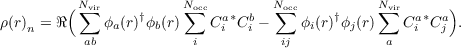
Difference densities based on natural transition orbitals If the excitation vectors have been obtained starting from a GHF reference, the NTOs are complex and contain contributions from both spin function. Moreover, the transitions are usually dominated by two NTOs at least. Thus, the interpretation of 2c-NTOs may become difficult. To get a simple picture of the transition at hand still, approximate difference densities can be computed according to
 | (18.3) |
The first term corresponds to the increase of the occupation of the virtual NTOs, while the second
term corresponds to the decrease of the occupation of the occupied NTOs.
This approximate difference density is available for excitation vectors obtained with the
following methods: CCS/CIS, CIS(D∞), ADC(2) and CC2. Symmetry other than C1 is
currently not supported. Note that the approximate difference densities are based on the
same approximations as the NTOs, namely ignoring correlation and double excitation
contributions.
From excitation amplitudes computed with the ricc2 program the approximate difference densities are computed with ricctools. E.g. using the right eigenvectors for the second singlet excited state in irrep 1:
ricctools -diffden CCRE0-1--1---2
This resulting density file can be visualized using the analysis mode of the ricc2 program as described in Section 10.3.3, e.g. by adding the following lines to the control file
and running
Fit of charges due to the electrostatic potential: $esp_fit fits point charges at the positions of nuclei to electrostatic potential arising from electric charge distribution (for UHF cases also for spin density, also possible in combination with $soghf). For this purpose the ("real") electrostatic potential is calculated at spherical shells of grid points around the atoms. By default, Bragg-Slater radii, rBS, are taken as shell radii.
A parametrization very close to that suggested by Kollman (a multiple-shell model with shells of radii ranging from 1.4*rvdW to 2.0*rvdW, rvdW is the van-der-Waals radius; U.C. Singh, P.A. Kollman, J. Comput. Chem. 5(2), 129-145 (1984)) is used if the keyword is extended:
$esp_fit kolman