Both the OEP-EXX and LHF methods can be used in spin–restricted closed–shell and spin–unrestricted open–shell ground state calculations. Both OEP-EXX and LHF are parallelized in the OpenMP mode.
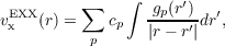
In the present implementation the OEP-EXX local potential is expanded as [223]:
|
| (19.6) |
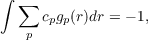
where gp are gaussian functions, representing a new type of auxiliary basis-set (see directory xbasen). Inserting Eq. (19.6) into Eq. (19.2) a matrix equation is easily obtained for the coefficient cp. Actually, not all the coefficients cp are independent each other as there are other two conditions to be satisfied: the HOMO condition, see Eq. (19.4), and the Charge condition
 | (19.7) |
which ensures that vxEXX(r) approaches -1∕r in the asymptotic region. Actually Eq. (19.6) violates the condition (19.5) on the HOMO nodal surfaces (such condition cannot be achieve in any simple basis-set expansion).
Note that for the computation of the final KS Hamiltonian, only orbital basis-set matrix elements of vxEXX are required, which can be easily computes as three-index Coulomb integrals. Thus the present OEP-EXX implementation is grid-free, like Hartree-Fock, but in contrast to all other XC-functionals.
In the LHF implementation the exchange potential in Eq. (19.3) is computed on each grid-point and numerically integrated to obtain orbital basis-sets matrix elements. In this case the DFT grid is needed but no auxiliary basis-set is required. The Slater potential can be computed numerically on each grid point (as in Eq. 19.3) or using a basis-set expansion as [219]:
Here, the vector χ(r) contains the basis functions, S stands for the corresponding overlap matrix, the vector ua collects the coefficients representing orbital a, and the matrix K represents the non-local exchange operator xNL in the basis set. While the numerical Slater is quite expensive
but exact, the basis set method is very fast but its accuracy depends on the completeness of the
basis set.
xNL in the basis set. While the numerical Slater is quite expensive
but exact, the basis set method is very fast but its accuracy depends on the completeness of the
basis set.
Concerning the correction term, Eq. (19.3) shows that it depends on the exchange potential itself. Thus an iterative procedure is required in each self-consistent step: this is done using the conjugate-gradient method.
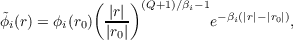
Concerning conditions (19.4) and (19.5), both are satisfied in the present implementation. KS occupied orbitals are asymptotically continued [227] on the asymptotic grid point r according to:
 | (19.9) |
where r0 is the reference point (not in the asymptotic region), β =  and Q is the molecular
charge. A surface around the molecule is used to defined the points r0.
and Q is the molecular
charge. A surface around the molecule is used to defined the points r0.
