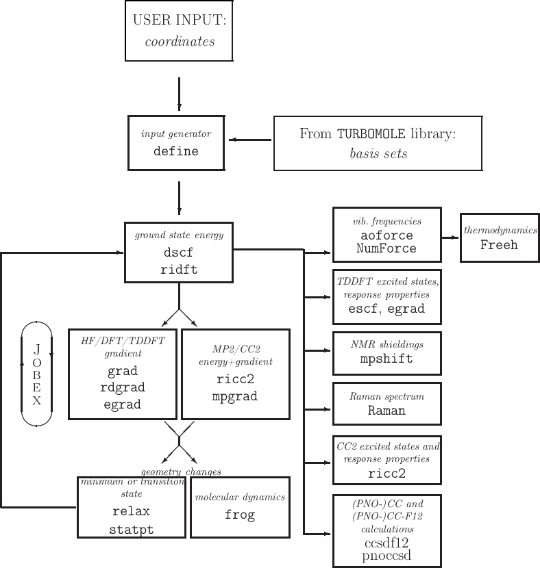
Figure 3.1: The modules of Turbomole and the main data flow between them.
The easiest way to start with TURBOMOLE is to use the free graphical user interface TmoleX which is part of every TURBOMOLE distribution. Please install TmoleX on your local desktop computer and avoid running the GUI on remote machines using remote desktop tools like X11. If you do not have a local version of TmoleX, consider to download and use the free version which is able to generate input, to run TURBOMOLE jobs on external (Linux) boxes and to visualize the results - download is available from here: http://www.cosmologic.de/support-download/downloads/tmolex-client.html
A detailed tutorial for the usage of TURBOMOLE on the command line can be found in the
DOC directory of your TURBOMOLE installation or on the web site of COSMOlogic, see
http://www.cosmologic.de/
In General:
All TURBOMOLE modules need the control file as input file. The control file provides directly or by cross references the information necessary for all kinds of runs and tasks (see Section 20).
The define module (program) generates in a step by step manner and interactively the control file: Coordinates, atomic attributes (e.g. basis sets), MO start vectors (using the charge of the molecule) and keywords specific for the desired method of calculation. We recommend generating a set of Cartesian coordinates for the desired molecule using special molecular design software and converting this set into TURBOMOLE format (see Section 21.2) as input for define. Alternatively the graphical user interface TmoleX can be used to import and/or build molecules.
A straightforward way to perform a TURBOMOLE calculation from scratch is as follows:
If that was a too quick and dirty chapter, please read the TURBOMOLE Tutorial in the DOC directory of your local TURBOMOLE installation. It explains step by step the generation of input with define and how to run calculations on the command line.
All calculations are carried out in a similar way. First you have to run define to obtain the control file or to add/change the keywords you need for your purpose. This can also be done manually with an editor. Given a bash and a path to $TURBODIR/bin/[arch] (see installation, Chapter 2) you call the appropriate module in the following way (e.g. module dscf):
nohup dscf > dscf.out &
nohup means that the command is immune to hangups, logouts, and quits. & runs a background command. The output will be written to the file dscf.out. Several modules write some additional output to the control file. For the required keywords see Section 20. The features of TURBOMOLE will be described in the following section.
Energy calculations may be carried out at different levels of theory.
use modules dscf and grad or ridft and rdgrad to obtain the energy and
gradient. The energy can be calculated after a define run without any
previous runs. dscf and grad need no further keywords ridft and rdgrad only
need the keyword $rij. The gradient calculation however requires a converged
dscf or ridft run.
DFT calculations are carried out in exactly the same way as Hartree–Fock
calculations except for the additional keyword $dft. For DFT calculations
with the fast Coulomb approximation you have to use the modules ridft and
rdgrad instead of dscf and grad. Be careful: dscf and grad ignore RI–K
flags and will try to do a normal calculation, but they will not ignore RI–J flags
($rij) and stop with an error message. To obtain correct derivatives of the
DFT energy expression in grad or rdgrad the program also has to consider
derivatives of the quadrature weights—this option can be enabled by adding
the keyword weight derivatives to the data group $dft.
For a semi-direct dscf calculation (Hartree–Fock or DFT) you first have to perform a statistics run. If you type
stati dscf
nohup dscf > dscf.stat &
the disk space requirement (MB) of your current $thime and $thize combination will be computed and written to the data group $scfintunit size=integer (see Section 20.2.7). The requirement of other combinations will be computed as well and be written to the output file dscf.stat. The size of the integral file can be set by the user to an arbitrary (but reasonable) number. The file will be written until it reaches the given size and dscf will continue in direct mode for the remaining integrals. Note that TURBOMOLE has no 2GB file size limit.
MP2 calculations need well converged SCF runs (the SCF run has to be done with
at least the density convergence $denconv 1.d-7, and $scfconv 7 as described in
Section 20). This applies also to the spin-component scaled (SCS and SOS) and
explicitly-correlated (F12) variants of MP2. For MP2 and MP2-F12 calculations in
the RI approximation use the ricc2 or pnoccsd modules. The module
mpgrad calculates the conventional (non-RI and non-F12) MP2 energy its gradient
(only recommended for test calculations). The input can be prepared with the mp2,
cc, or pnocc menu in define.
Single point excited state energies for CIS, TDHF, and TDDFT methods can be
calculated using escf. Excited state energies, gradients, and other first order
properties are provided by egrad. Both modules require well converged ground state
orbitals.
The module ricc2 calculates beside MP2 and CC2 ground state energies also CIS
(identical to CCS), CIS(D), CIS(D∞), ADC(2) or CC2 excitation energies
using the resolution-of-the-identity (RI) approximation. Also available are
spin-component scaled (SCS and SOS) variants of the second-order methods
CIS(D), CIS(D∞), ADC(2) or CC2. Excited state gradients are available
at the CCS, CIS(D∞), ADC(2), and CC2 levels and the spin-component
scaled variants of the latter three methods. In addition, transition moments
and first-order properties are available for some of the methods. For more
details see Section 10. The input can be prepared using the cc menu of
define.
Coupled-Cluster methods beyond CC2 as CCSD and CCSD(T) and Møller-Plesset
perturbation theory beyond MP2 and explicitly-correlated F12 variants thereof
are since Release V7.0 implemented in the ccsdf12 program. The F12
variants of these methods have a much faster basis set convergence and are
therefore more efficients. We recommend in particular CCSD(F12*) and
CCSD(F12*)(T). Excitation energies are only available for (conventional)
CCSD.
See Section 1.4 for the functionality and Section 20 for the required keywords of the modules dscf, ridft, mpshift, escf, and ricc2.
See Figure 3.1.