17.5 Polarizable embedding calculations

Polarizable embedding (PE) calculations are a based on a hybrid model of quantum mechanics and molecular mechanics (QM/MM) in which the classical region is represented by an electrostatic potential with up to octupole moments and induced point dipole moments. The main improvement over the more common QM/MM approaches without polarizable MM sites can be found for the description of electronic excitations but also for any other process which causes a significant change in the QM density and which is accompanied by a fast response of the environment.

In TURBOMOLE, only ground state energies computed with the dscf, ridft, and ricc2 module and electronic excitation properties based on RI-CC2 are implemented. The general theory is presented in ref.  [208] and [209], the PERI-CC2 model and the TURBOMOLE implementation is described in ref.  [210].

17.5.1 Theory

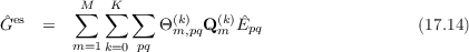
In the following, only the most important ideas are presented and discussed with a focus on the PERI-CC2 model. The essential concept is the introduction of an environment coupling operator Ĝ(D^CC)

with the electrostatic contribution

and the polarization contribution

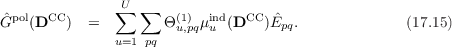
Here, Θ_m,pq^(k) are multipole interaction integrals of order k and μ_u^ind are the induced dipoles which can be obtained from the electric field F_u and the polarizability α_u at a site u:

(17.16)

Because the induced dipoles depend on the electron density and vice versa, their computations enter the self-consistent part of the HF cycle. Introducing Ĝ(D^CC) into standard equations for the HF reference state and the CC2 equations leads to a general PE-CC2 formulation. To maintain efficiency, a further approximation has been introduced which makes the operator only dependent on a CCS-like density term. These general ideas define the PERI-CC2 model and allow to formulate the corresponding Lagrangian expression

from which all PERI-CC2 equations including the linear response terms may be derived. Note that the dependency on the density couples the CC amplitude and multiplier equations for the ground state solution vector.

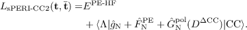
This coupling is avoided by the simplified polarizable embedding method (sPE) described in ref.  [211].

(17.18)

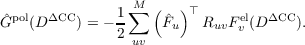
The subscript N indicates that the operator is normal ordered with respect to the Hartree–Fock state. Here, a polarization operator Ĝ^pol(D) was introduced,

(17.19)

which depends on the elements of the difference density matrix D^ΔCC. These are defined as

(17.20)

hence, they do not depend on the Lagrangian multipliers.

17.5.2 Computational details: SCF calculations

To carry out a PE-SCF calculation with the DSCF or RIDFT module, you have to specify the following in the control file:

length unit

specifies the unit for the MM site coordinates (use AA or AU)

no. MM sites

the amount of MM sites (length of the list)

order k

the order of multipoles used (0: point charges, 1: dipole moments, 2: quadrupole moments, 3: octupole moments)

order pol

the treatment of polarizabilities (0: none, 1: isotropic, 2: anisotropic)

length exclude list

number of elements in the exclude list

list of MM sites

each MM sites is described on one line, entries separated by blanks; first entry is the exclude list of with as much elements as defined in the head line (If the first element in the exclusion list of one site occurs in the exclude list of another site, they do not contribute to each others polarization); next follows the MM site coordinates in (x,y,z positions), the point charge, the dipole moment (for k ≥ 1, x,y,z component), the quadrupole moment (for k ≥ 2, xx, xy, xz, yy, yz, zz component), the octupole moment (for k = 3, xxx, xxy, xxz, xyy, xyz, xzz, yyy, yyz, yzz, zzz component), the polarizability ( one component for pol-order 1, xx, xy, xz, yy, yz, zz component for pol-order 2)

An example for a polarizable embedding with coordinates given in Å, point charges and isotropic polarizabilities:

All values are given in atomic units (except coordinates if stated otherwise). These data are mandatory. An alternative input format can also be used by specifying daltoninp as option on the $point_charges line. The format is completely compatible with the current Dalton 2015 input format (The definition can be found in the manual from http://daltonprogram.org/www/documentation.html. See there for more information).

In addition, you can specify further options on the same line as the $point_charges flag. These are:

• rmin=<float>: minimum distance between an active MM site and any QM center (in a.u.), treatment is handle by option iskip, (DEFAULT: 0.00 a.u.)
• iskip=(1,2) : treatment of too close MM sites
  • (1) zeroing all contributions
  • (2) distribute values to nearest non-skipped MM site (DEFAULT)
• rmax=<float>: maximum distance between an active MM site and QM center of coordinates (in a.u.), sites too far away are skipped (zeroed) (DEFAULT: 1000.00 a.u.)
• nomb: no treatment of many body effects between induced dipoles (all interaction tensors on the off-diagonal of the response matrix are set to Zero); works best with isotropic polarizabilities, speeds up calculations (especially for large response matrices), has reduced accuracy, not well tested so far
• longprint=(1,2,3): sets a flag for additional output
  • (1) print all MM site input information
  • (2) additionally: print all induced dipoles due to nulcei/multipole/electron electric filed
  • (3) additionally: print response matrix
• file=<input file>: specifies a file from which the data group $point_charges is read. Note that all options which are following on the line in the control file are then ignored because reading continues in the input file (But here, further options can be specified after the $point_charges flag). The file has to start with $point_charges as top line and should be finished with $end
• ccdens: activates the simplified polarizable embedding method

Limitations with respect to standard SCF computations:

• In PE-SCF computations, symmetry cannot be exploited.
• PE-SCF computations do not work in parallel (MPI parallelization).
• For two-component all-electron calculations, the decoupling of the embedding potential is neglected, i.e. it is affected by a picture-change error just like the two-electron integrals.

The energy of a PE-SCF calculation printed in the output contains the following terms:

(17.21)

Here, E_QM is the energy of the quantum mechanical method of your choice, E_QM∕MM,es the electrostatic interaction energy between the QM and the MM region, and E_pol the energy gain due to the total of induced dipole moments. If necessary, missing terms can be computed without knowledge of the electron distribution.

At the moment, TURBOMOLE does not offer the possibility to generate the necessary potentials or to create a potential file from a set of coordinates. Embedding potentials can be obtained from literature or generated by approaches like the LoProp method. [212] Atom centered polarizabilities are also available from other methods or from experiment. Finally, there are some polarizable force fields which, in principle, can be used for the PE method (for example, the AMOEBA force field).

17.5.3 Computational details: PERI-CC2 calculations

Apart from the definition of the embedding described above, the input for PERI-CC2 calculations is the same as without polarizable embedding.

There are several limitations for the use of PERI-CC2:

• only ground state energies, excitation energies and transition moments are supported (no other properties or gradients and so on)
• no other wave function model than CC2 is supported
• no use of symmetry
• no MPI parallelization is available (but SMP binaries work)
• open-shell systems are not covered (exception: two-component references)