There are several possibilities to visualize structures, vibrational frequencies, molecular orbitals, densities and a large number of properties.
The easiest one is to use the graphical user interface of TURBOMOLE TmoleX. TmoleX is either included in your TURBOMOLE distribution or can be downloaded for free from the COSMOlogic web site TmoleX client version. Use the COSMObuild part of TmoleX to read in the 3D data from file (plt or plv format).
The tool t2x can be used to convert the atomic coordinates stored in the $grad and $coord data groups into the xyz-format, which is supported by most viewers, e.g. jmol. Typing
in a directory containing the control file generates a series of frames using the information in $grad. Note t2x writes to standard output which here is redirected to a file. If you are only interested in the most recent structure, type
which only extracts the information on $coord.
Note that the easiest way to visualize orbitals, densities and electrostatic properties is to use the graphical user interface TmoleX.
There are several other possibilities to visualize molecular orbitals or densities.
The molden option in the export menu of proper converts the MO and geometry information to the molden format. Alternatively one can use the conversion program tm2molden, which is interactive and self-explanatory. The generated file can be read in by the molden program (see molden web site).
For larger systems this may become very time-consuming, as plotting data (values on grids) are calculated by the respective programs (e.g. molden). It is more efficient to calculate the data for plots (MO amplitudes, densities, etc.) with TURBOMOLE and to use a visualization tool afterwards, a way, that is described in the following.
Calculation of data on grids to be used for plots with visualization tools (e.g. gOpenMol, available via gopenmol download) can be generated with the options in the grid menu of proper. Alternatively one can use the keyword $pointval in combination with the -proper option. This keyword is obeyed by all TURBOMOLE program that generate densities as dscf, ridft, rimp2 mpgrad, ricc2 (see Section 10.3.3) and egrad. Note, that with -proper and $pointval all of the following quantities may be calculated simultaneusly, and that for programs dscf, ridft, rimp2 and mpgrad the density matrix generating steps may be skipped by typing "<program> -proper".
Electron densities The option dens in the grid menu of proper or with the above mentioned programs setting of the keyword
$pointval dens
or simply
$pointval
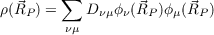
results in the calculation of densities
|
| (18.4) |
on an orthogonal grid of point  P. The size of the grid is automatically adjusted to
the size of the molecule and the resolution is adjusted to yield acceptable plots (for
specification of non-default grid types (planes, lines) and non-default output formats see
Section 20.2.25).
P. The size of the grid is automatically adjusted to
the size of the molecule and the resolution is adjusted to yield acceptable plots (for
specification of non-default grid types (planes, lines) and non-default output formats see
Section 20.2.25).
The names of the output files are:
total density (UHF: α density plus β density )
spin density (α density minus β density )
MP2 density
MP2 spin density
differential density for excited state
differential spin density for excited state
The .plt files may be visualized with gOpenMol; the file coord.xyz, which is also necessary for gOpenMol, is generated by the above programs, if $pointval is set in the control-file.
For two-component wavefunctions (only module ridft with $soghf is set): Total density is on file td.plt like for one-component wave functions; this is also true for all other quantities depending only on the density matrix (electrostatic potential etc.). sd.plt contains the absolute value of the spin vector density, which is the absolute value of the following vector:
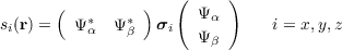 |
$pointval fmt=txt
leads to a file containing the spin density vectors, which can be used by gOpenMol. It is advisable to choose ca. one Bohr as the distance between two gridpoints. The options for visualizing two-component wavefunctions are not yet available in the proper program.
Available output formats: To get a list of the available output formats of the proper program invoke the format option with the flag help. For the direct generation of graphics output different formats are available for 3D and 2D plots. They depend furthermore on the graphics libraries linked to proper. Use the format option with the help flag for a 2D and a 3D grid to get the list of formats available for the two cases. For the output formats available in combination with -proper keyword to export data on grids see Section 20.2.25.
Electrostatic potentials In an analogous way electrostatic potentials can be calculated on grids. The option ($pointval) pot leads to the calculation of the electrostatic potential of electrons and nuclei (and external constant electric fields and point charges Q if present).
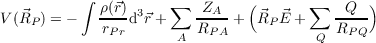 | (18.5) |
In order to prevent the calculation of singularities at the positions of nuclei, for gridpoints that are closer to a nucleus than 10-6 a.u. the charge of the respective nucleus is omitted in the calculation of the electrostatic potential for these points. The output files are termed tp.plt, sp.plt, etc.
Electric fields (as derivatives of potentials) are calculated with ($pointval) fld. The absolute values of electric fields are written to files tf.plt, sf.plt, etc. For non-default grid types and outputs that allow also for displaying of components of electric fields see Section 20.2.25.
Exchange-correlation potentials (Only for DFT) Computation of the Kohn-Sham exchange-correlation potential on a grid is requested with
This functionality is not (yet) available in the proper program.
Canonical molecular orbitals. Visualization of molecular orbitals, i.e. generation of .plt-files containing amplitudes of MOs i
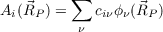 | (18.6) |
or in the two-component case
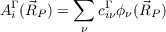 | (18.7) |
with Γ as a part of the coefficient matrix (Re(α), Im(α), Re(β), Im(β)), is achieved e.g. by ($pointval) mo 10-12,15. This triggers the calculation of amplitudes for the MOs/spinors 10-12 and 15 on the grid. The numbering of MOs refers to that you get from the first column of the output of the tool Eiger, the one for spinors refers to the file EIGS. The filenames contain the type of the irreducible representation (irrep) of the MO, the current number within this irrep and in case of UHF calculations also the spin, e.g. 2a1g_a.plt contains amplitudes for the second alpha-spin MO of a1g type. For more-dimensional irreps columns are written to separate files, e.g. 1t2g1_a.plt, 1t2g2_a.plt and 1t2g3_a.plt contain the amplitutes of the three columns of the first irrep (alpha spin) of type t2g.
Two-component wavefunctions (only module ridft and only if $soghf is set): By default only the density of the chosen spinors is written in files named e.g. 10a_d.plt. Visualization of the amplitudes of the different spinor parts is achieved e.g. by
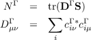
$pointval mo 10-12,15 minco real,
where real is a plotting threshold that may take values between zero and one. The corresponding part Γ of the spinor (Re(α, Im(α, Re(β, Im(β)) will be written to file, if NΓ (see below) is larger than that threshold.
Localised molecular orbitals If one has generated localized molecular orbitals (LMOs, see above) they can also be visualized.
as an example, leads to calculation of amplitudes for LMOs 3-6 and 8. The coefficients are read from file lmos (UHF: lalp and lbet), the numbering refers to the output from the localization section. For an UHF case the β spinorbitals get an offset of NMO, where NMO is the total number molecular orbitals for each spin case. If one has e.g. 22 orbitals per spin case and is interested in plotting the first 3 β-type LMOs only, one have to type
$pointval lmo 23-25
Natural molecular orbitals for two-component wavefunctions (only module ridft and only if $soghf is set): In two-component calculations it is often useful to visualize natural molecular orbitals. In contrast to one-component calculations the occupation numbers are no longer close to zero, one or two, but can take any value between zero and two. Therefor
$natural orbitals file=natural
$natural orbital occupation file=natural
has to be set additionally to $soghf (also possible via define).
By setting
$pointval nmo 9
in control-file a gOpenMol-compatible file named nmo_9.plt is written which can also be visualized with TmoleX.
Natural atomic orbitals If one has generated natural molecular orbitals (NAOs, see above) they can be visualized with the following command in the control file:
where the numbers of the NAOs are in the output of the population analysis.
Natural transition orbitals If natural transition orbitals (NTOs) for electronic excitations are available in files named nto_nocc and nto_vir for, respectively, the occupied and virtual NTOs, plot files for visualizing them can be generated by setting
This will generate plot files for the first five occupied and virtual NTOs. The plot file are named nto_vir_n.plt, where n is the NTO index.
Non-default grids are decribed in detail in Sections 20.2.25. In the proper program non-default grids can be specified with the grid option. Calculation of the above quantities at single points is needed quite often, thus an example is given here.
calculates densities at points (7,5,3), (0,0,7) and (1,2,3). Output is (x,y,z, density), output file suffix is .xyz.
We note in passing that calculation of electrostatic potential at positions of nuclei may be used as an efficient tool to distinguish atoms of similiar atomic numbers thus providing a complement to X-Ray Structure Analysis (details see ref. [218]).